
Concepts of Linear Systems and Convolution
Discrete Convolution is a tool to build any linear and shift invariant filter. The equation for the convolution, g(x), of the sequence f(x) with the convolution kernel h(x) is

h(x) is also called the impulse response, Point Spread Function PSF, window kernel, window mask, window, filter, or template. This formula can be easily extended to the 2D case.
We normally show the region of support of the convolution kernel. That is, the region where the kernel values are valid. The kernel values are zero outside the region of support.
There are two main types of convolution, depending on how we define the data: Linear Convolution and Circular Convolution.
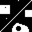 ------

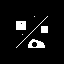
Left:original image f; Right: kernel h
 -
-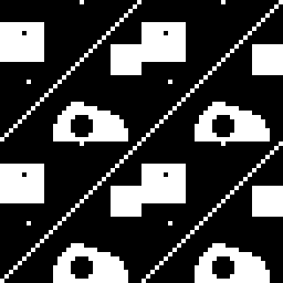
Left: zero outside (for linear convolution),
Right: periodic (for circular convolution
 -
-
Left: 3x3 kernelfor linear convolution,
Right: 3x3 kernel for circular convolution (periodic with same period as the image)
When we define a convolution kernel, we do not always we have the origin of its coordinates positioned at the top left corner of its region of support. Normally, there is a shift in the resultant image if the origin of the convolution kernel is not at the center of its region of support. A simple name for the origin is "sweet spot".
 linear *
 =
=
 circular *
 =
=
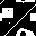
Circular Convolution. Note the output with same dimensions.
 linear *
 =
=
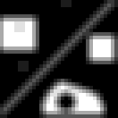
 circular *
 =
=
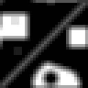
Circular Convolution.
 linear *
 =
=
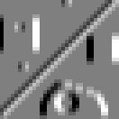
 circular *
 =
=
Circular convolution.
Observe that if there is an isolated point (impulse) in the input image then the kernel appears reproduced in the filtered or output image.